Decomposition

A spectrum does not only consist of well separated peaks but they often appear as multiplets (a line in a spectrum composed of a group of related lines). For the decomposition of multiplets a fit must be used. Therefore a description of the observed line shapes is necessary. Otherwise it is impossible to find the correct number of overlapping lines and to obtain a good description of the spectrum.

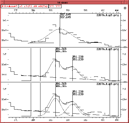
As an example what can happen if you fit a multiplet in the wrong way figure 4.5 on page

shows in its upper pane a quickfit. As you can see, it can not decompose the two peaks. In the middle pane a normal fit has been performed with two peakmarkers set and in the lower pane the decomposition is shown. You can show or hide the decomposition with the commands:

**Figure 4.5:** Graphic-display window with a ²²⁰ Th spectrum loaded and a fit attached. **Upper:** A quickfit has been performed. The peaks are not decomposited. **Middle:** A normal fit is performed with two peaks marked. **Lower:** The fit function and its decomposition is shown.
$\begin{figure} \begin{center} \leavevmode \epsffile {pictures/fit-demo-multiplet.ps} \end{center}\end{figure}$

TV uses a modified gaussian with left tail and right tail and an underlying step. Parameters of the gaussian are position, volume and width as well as left and right tail and finally width and height of the step (see section D.1 p.

). These seven parameters are associated with each peak fitted. To reduce the number of parameters it is possible to use calibrations for single parameters or to correlate them, e.g. to equal widths. Step and tail parameters sometimes can be neglected. The background parameters can be simultaneously fitted with the peaks or can be fixed in advance by a fit in separate background regions. To select the peak function or background function to be used or whether parameters are to be fitted or not use the following commands (for all fit function and fit parameter commands see section 6.4.7 on page

and section 6.4.12 on page

To activate a certain peak function (by default continuous-exp-tail/arctan-step is active) enter:

You can generally set parameters to a value and hold this value, i.e. disallow TV to fit the parameter or set the parameter free and allow TV to fit it. If you do not want TV to fit a parameter after you set it you should set it to hold.

and the exponential term is activated by setting the parameter FAC to nonzero with:

All parameters which can be influenced by the fit parameter command are listed in table 4.7 on page

Table 4.7: Fit parameters and their meaning.
Parameter Meaning

background Degree of background function.

exponent-background Scaling of exponential term (see section D.2 p. ).

factor-background Factor of exponential term (see section D.2 p. ).

position Position.

sh Height of step.

sw Width of step.

tl Left tail.

tr Right tail.

volume Volume.

width Width.

It is important to choose the optimal procedure to optimize the parameters. The correct fit function gives the expectation value for the contents of each channel fitted. Since the measured values follow a probability distribution, their probability with respect to the expected function is known for each channel. For a certain set of parameters a total probability can be calculated as product of these channel probabilities. The optimal set of parameters is assumed to be most likely. It is determined by searching the maximum of this product in dependence of the free parameters (maximum likelihood).

**Table 4.7:** Fit parameters and their meaning.
Parameter	Meaning
background	Degree of background function.
exponent-background	Scaling of exponential term (see section D.2 p. ).
factor-background	Factor of exponential term (see section D.2 p. ).
position	Position.
sh	Height of step.
sw	Width of step.
tl	Left tail.
tr	Right tail.
volume	Volume.
width	Width.

By default it is assumed that the channel contents follow a gaussian distribution. In this case maximum likelihood is equivalent to the commonly used

χ

² -minimization (see section D.3 p.

). Unfortunately this is not applicable if the expectation values for the contents of single channels are in the order of one. In this case the values are described by a poisson distribution. Obviously the fit function misestimates the contents of the spectrum. This does not depend on the integral of the fitted data but only on the amplitudes, i.e. it does not matter how large the fitted region is.

Besides the

χ

² -minimization TV can do the maximization of the poisson distribution (see section D.3 p.

). The results determined by this method are correct as long as the spectra have only be incremented or added. For normalized or subtracted spectra the variance of the data following the poisson distribution is not defined and therefore this method is not usable for those spectra. For data distributed according to the gaussian distribution these operations are possible. As a conclusion from the above one can say that none of the measure functions determines correct results, if for example gates with low statistics have been subtracted.