Graphic window types

    TV offers several types of windows suitable for special purposes.

First there is the basic window type simple which consists of just one pane. You can use it to display an arbitrary number of spectra.

There is one special window of window type simple, the plot window. Since the default frame width for the left and right side is not large enough to see the scale's inscriptions on your plot you can enlarge them (see section 4.6 p. ) or create a new window named plot which is suitable for the plotting of spectra.

tv$>$ window create simple plot

Besides the simple window there are three different paned windows, the xy-, x- and y-paned. They are composed of one or more panes, which are arranged one above the other. All panes share a common status line. These window types provide a y-scale per pane and a total of two x-scales. In an xy-paned window the x-scales are independent as well as the y-scales. The scale at the top of the window belongs to the uppermost spectrum shown and the one at the bottom to the lowest. So with more than two panes, you have spectra without x-scale. In x- or y-paned windows, the x-scales are coupled to all spectra shown. So if you set x-view markers with Spacebar in one pane and expand with e, the viewport in all panes will be changed. In a y-paned window (see figure 4.2 p. ) all y-scales are coupled, too.

tv$>$ window create {paned $|$ xpaned $|$ ypaned} name$>$ number$>$

Paned windows are good means for the comparison of many spectra. For example you can create an x-paned window for the comparison of four distances of a lifetime experiment with the command:

tv$>$ window create xpaned lifetime 4

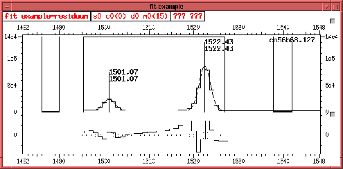
The remaining window types are composed of two graphic subwindows. The fit window is an x-paned window in which lower pane the residuum of the fit is shown. The cut window has a small subwindow in its upper right corner where the position of the cut marker in the projection is shown (see figure 2.5 p. ).

tv$>$ window create {fit $|$ cut} name$>$

Figure 4.1 on page shows an example for the fit window that was created with the command:

tv$>$ window create fit ``fit example''

In the lower pane the residuum is displayed.

  

Figure 4.1: A fit of two peaks in a $56$Co spectrum in the special fit window. In the lower pane the residuum is displayed.

To delete the graphic window named ``fit example'' use the command:

tv$>$ window delete ``fit example''